

Code as a Crime Scene
by Adam Tornhill, November 2013
The following article was the starting point for my new book - Your Code as a Crime Scene - published by the Pragmatic Programmers. Check it out!
Code as a Crime Scene - the Article
Technical challenges rarely come in isolation. In any large-scale project they interact with social and organizational aspects. To address that complexity we need to look beyond the current structure of the code. We need strategies to identify design issues, a way to find potential suspects like code smells and team productivity bottlenecks. Where do you find such strategies if not within the field of criminal psychology?
Inspired by modern offender profiling methods from forensic psychology we'll develop techniques to utilize historic information from our version-control systems to identify weak spots in our code base. Just like we want to hunt down criminals in the real world, we need to find and correct offending code in our own designs.
The maintenance puzzle
Maintenance is a challenge to every software project. It's the most expensive phase in any product's lifecycle consuming approximately 60 percent of the cost. Maintenance is also different in its very essence when compared to greenfield development. Of all those maintenance money, a whole 60 percent are spent on modifications to existing programs (Glass, 2002).
The immediate conclusion is that if we want to optimize any aspect of software development, maintenance is the most important part to focus on. We need to make it as cheap and predictable as possible to modify existing programs. The current trend towards agile project disciplines makes it an even more urgent matter. In an agile environment we basically enter maintenance mode immediately after the first iteration and we want to make sure that the time we spend in the most expensive lifecycle phase is well-invested.
So is it actually maintenance that is the root of all evil? Not really. Maintenance is a good sign – it means someone's using your program. And that someone cares enough to request modifications and new features. Without that force, we'll all be unemployed. I'd rather view maintenance as part of a valuable feedback loop that allows us to continuously learn and improve, both as programmers and as an organization. We just have to be able to act on the feedback.
The typical answer to that maintenance puzzle is refactoring (Fowler, 1999). We strive to keep the code simple and refactor as needed. Done by the book, refactoring is a disciplined and low-risk investment in the code base. Yet, many modifications require design changes on a higher level. Fundamental assumptions will change and complex designs will inevitably have to be rethought. In limited and specific situations refactoring can take us there in a controlled series of smaller steps. But that's not always the case. Even when it is, we still need a sense of overall direction.
Intuition doesn't scale
Since the 70's we have tried to identify complexity and quality problems by using synthetic complexity measurements (e.g Halstead (Halstead, 1977) or McCabe (McCabe, 1976) complexity measures). It's an approach that has gained limited success. The main reason is that traditional metrics just cannot capture the complex nature of software.
If complexity metrics don't work, at least not to their full promise, what's left for us? Robert Glass, one of my favorite writers in the software field, suggests intuition (Glass, 2006).
Human intuition is often praised as a gift with mystical, almost magical qualities. Intuition sure is powerful. So why not just have our experts glance at our code and pass an immediate verdict on its qualities and virtues? As we're about to discover, intuition has its place. But that place is more limited than my previous reference to Robert Glass suggests.
Intuition is largely an automatic psychological process. This is both a strength and a weakness. Automatic process are unconscious cognitive processes characterized by their high efficiency and ability to make fast and complex decisions based on vast amounts of information. But efficiency comes at a price. Automatic processes are prone to social and cognitive biases.
Even if we somehow manage to avoid those biases, a task that is virtually impossible for us, we would still have a problem if we rely on intuition. Intuition doesn't scale. No matter how good a programmer you are, there's no way your expertise is going to scale across hundreds of thousands or even million lines of code. Worse, with parallel development activities, performed by different teams, our code base gets another dimension too. And that's a dimension that isn't visible in the physical structure of the code.
A temporal dimension of code
Over time a code base matures. Different parts stabilize at different rates. As some parts stabilize others become more fragile and volatile which necessities a shift in focus over time. The consequence is that parts of the code base may well contain excess complexity. But that doesn't mean we should go after it immediately. If we aren't working on that part, and haven't been for quite some time, it's basically a cold spot. Instead other parts of the code may require our immediate attention.
The idea is to prioritize our technical debt based on the amount of recent development activity. A key to this prioritization is to consider the evolution of our system over time. That is, we need to introduce a temporal axis. Considering the evolution of our code along a temporal axis allows us to take the temperature on its different parts. The identified hot spots, the parts with high development activity, will be our priorities.
This strategy provides us with a guide to our code. It's a guide that shows where to focus our cognitive cycles by answering questions like:
- What's the most complex spot in our software that we're likely to change next?
- What are the typical consequences of that change?
- Is is likely to be a local change or will other parts have to change too? I.e. can we predict the impact on related and seemingly unrelated modules?
In their essence, such open problems are similar to the ones forensic psychologists face. Consider a series of crimes spread out over a vast geographical area:
- Where can we expect the next crime to occur?
- What area is most likely to serve as home base of the offender?
- Are there any patterns in the series of crimes? I.e. can we predict where the offender will strike again?
Modern forensic psychologist and crime investigators attack these open, large-scale problems with methods useful to us software developers too. Follow along, and we'll see how. Welcome to the world of forensic psychology!
Geographical Profiling of Crimes: a 2 minutes introduction
Modern geographical profiling bears little or none resemblance to the Hollywood cliché of “profiling” as seen in movies. There the personality traits of an anonymous offender are read like an open book. Needless to say, there's little to no research backing that approach. Instead geographical profiling has a firm scientific basis in statistics and environmental psychology. It's a complex subject with its fair share of controversies and divided opinions (in other words: just like our field of programming). But the basic principles are simple enough to grasp in a few minutes.
The basic premise is that the geographical location of crimes contain valuable information. For a crime to occur, there must be an overlap in space and time between the offender and a victim. The locations of crimes are never random. Most of the time criminals behave just like ordinary, law abiding citizens. They go to work, visit restaurants and shops, maintain social contacts. During these activities, each individual builds a mental map of the geographical areas he visits and lives in. It's a mental map that will come to shape the decision on where to commit a crime.
The characteristic of a crime is a personal trade-off between potential opportunities and risk of detection. Most offenders commit their offenses close to home (with some variation depending on the type of offense and the environment). The reason is that the area close to home is also the area where the known crime opportunities have been spotted. As the distance to the home increases, there's a decline in crimes. This spatial behavior is known as distance decay. At the same time, the offender wants to avoid detection. Since he may be well-known in the immediate area around the home base, there's typically a small area where no crimes are committed.
Once a crime has been committed, the offender realizes there's a risk associated with an immediate return to that area. The typical response is to select the next potential crime target in the opposite direction. Over time, the geographical distribution of the crimes become the shape of a circle. So while the deeds of an offender may be bizarre, the processes behind them are rationale with a strong logic to them (Canter & Youngs, 2008). It's this underlaying dark logic that forms the patterns and allows us to profile a crime series. By mapping out the locations on a map and applying these two principles we're able to get an informed idea on where the offender has his home base.
Finally, a small disclaimer. Real-world geographical profiling is more sophisticated. Since psychologically all distances aren't equal the crime locations have to be weighted. One approach is to consider each crime location a center of gravity and mathematically weight them together. That weighted result will point us to the geographical area most likely to contain the home base of the offender, our hot spot. But the underlaying basic principles are the same. Simplicity does scale, even in the real world.
The geography of code
Geographical profiling does not point us to an exact location. The technique is about significantly narrowing the search area. It's all about highlighting hot spots in a larger geographical area. The profiling techniques are tools used to focus scarce manual efforts and expertise to where they're needed the most.
It's an attractive idea to apply similar techniques to software systems. Instead of trying to speculate about potential technical debt amongst thousands or perhaps million lines of code, geographical profiling would give us to a prioritized lists of modules, the hot spots, our top offenders. That leaves us with the challenge of identifying both a geography of code and a spatial movement within our digital creations. Let's start with the former.
Over the years there have been several interesting attempts to visualize large-scale software systems. My personal favorite is Code City (Code City) where software systems are visualized as cities. Each package becomes a city block, each class a building with the number of methods defining the height and the number of attributes defining the base of the building. Not only does it match the profiling metaphor; it's also visually appealing and makes large, monolithic classes stand out.
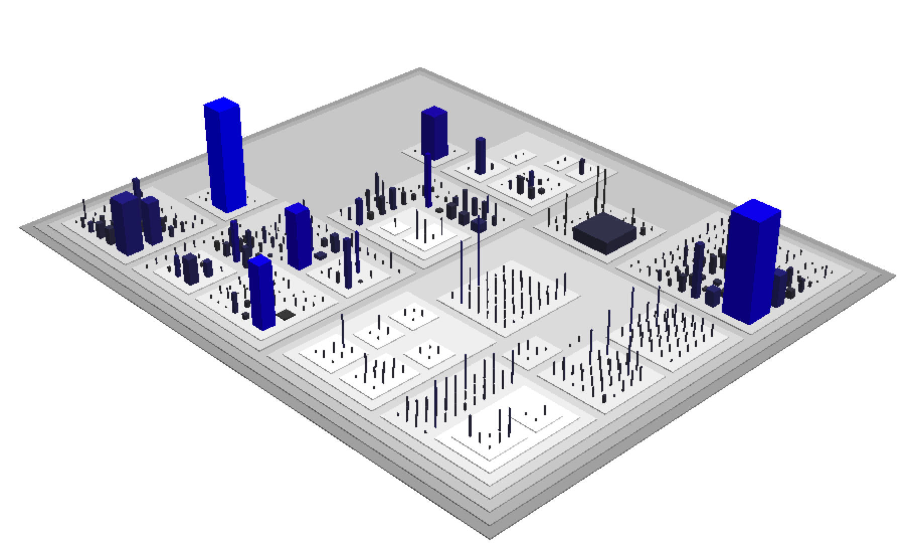
A geography of code as visualized by Code City. Each building represents a class with the number of methods giving the height and the attributes the base.
Visualizations may give us a geography, but the picture is no more complete than the metrics behind it. If you've been following along in this chapter, you'll see that we need another dimension - it's the overlap between code characteristics and the spatial movement of the programmers within the code that is interesting. That overlap between complex code and high activity are the combined factors to guide our refactoring efforts. Complexity is only a problem when we need to deal with it. In case no one needs to read or modify a particular part of the code, does it really matter if it's complex? Sure, it's a potential time bomb waiting to go off. We may choose to address it, but prefer to correct more immediate concerns first. Our profiling techniques allows us to get our priorities right.
Interaction patterns identify hot spots
Just like each crime provides the geographical profiler with valuable information, so does each code change in our system. Each change we make, each commit, contain information on how we as developers interact with the evolving system. The information is available in our version-control systems (VCS). The statistics from our VCS is an informational gold mine. Mining and analyzing that information provides us with quite a different view of the system:
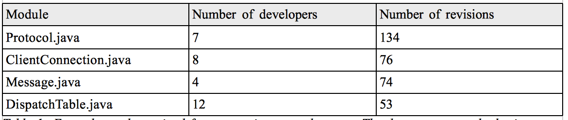
Example on data mined from a version-control system. The data servers as the basis to identify hot spots in our code base.
The VCS data is our equivalent to spatial movement in geographical profiling since it records the steps of each developer. The subset I chose to mine is derived from organizational metrics known to serve as good predictors of defects and quality issues (see for example Nagappan et al., 2008):
- Number of developers: The more developers working on a module, the larger the communication challenges. Note that this metric is a compound. As discussed below, the metric can be split into former employed developers and current developers to weight in potential knowledge drain.
- Number of revisions: Code changes for a reason. Perhaps because a certain module has too many responsibilities or because the feature area is poorly understood. This metric is based on the idea that code that has changed in the past is likely to change again.
In contrast to traditional metrics, organizational metrics carry social information. Depending on the available information, additional metrics may be added. For example, it's rare to see a stable software team work together for extended periods of time. Each person that leaves drains the accumulated knowledge. When this type of information is available, it's recommended to weight it into our analysis.
Together those metrics let us identify the areas of the system that are subject to particularly heavy development, the areas with lot of parallel development activity by multiple developers or the parts with the highest change frequency. In geographical profiling we combined the principles of distance decay and the circle hypothesis to predict the home base of an offender. In the same spirit we can visualize the overlap between traditional complexity metrics and our new organizational metrics:
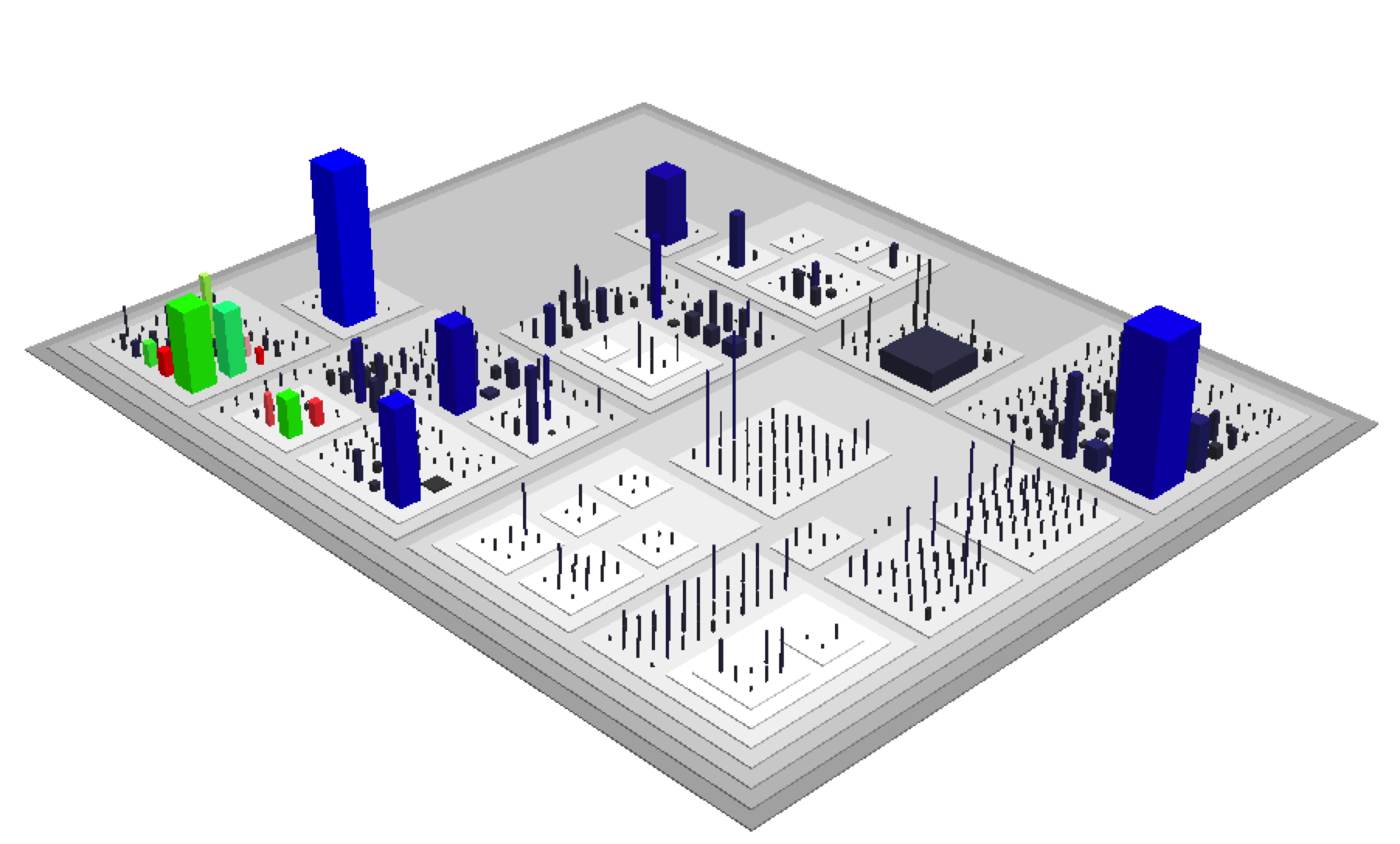
Custom color mark-up in Code City to highlight areas of intense parallel development by multiple programmers; the more intense the colors, the more activity.
The outcome of such hot spot analysis in code has often surprised me. Sometimes, the most complex areas are not necessarily where we spend our efforts. Instead, I often find several spread-out areas of intense development activity. With multiple developers crowding in those same areas of a code base, future quality issues and design problems will arise.
Emergent design driven by software evolution
Our crash-course in geographical profiling of crimes taught us how linking crimes and considering them as a related network allows us to make predictions and take possible counter steps. Similarly VCS data allows us to trace changes over series of commits in order to spot patterns in the modifications. The resulting analysis will allow us to detect subtle problems that go beyond what traditional metrics are able to show. It's an analysis that suggests directions for our refactorings based on the evolution of the code itself. The basis is a concept called logical coupling.
Logical coupling refers to modules that tend to change together. The concept differs from traditional coupling in that there isn't necessarily any physical software dependency between the coupled modules. Modules that are logically coupled have a hidden, implicit dependency between them such that a change to one of them leads to a predictable change in the coupled module. Logical coupling shows-up in our VCS data as shared commits between the coupled modules.
A temporal period for logical coupling
I've been deliberately vague in my definition of logical coupling. What do I really mean with "modules that tend to change together"? To analyze our VCS data we need to define a temporal period, a window of coupling. The precise quantification of that period depends on context.
In it's most basic form I consider modules logically coupled when they change in the same commit. Often, such a definition takes us far enough to find interesting and unexpected relationships in our system. But in larger software organizations that definition is probably too narrow. When multiple teams are responsible for different parts of the system, the temporal period of interest is probably extended to days or even weeks.
Analyzing logical coupling
At the time of writing there's limited tool support for calculating logical coupling. There are capable academic research tools available (Ambros, Lanza & Lungu, 2006), but AFAIK nothing in the open-source space. For the purpose of this article I've started to work on Code Maat, a suite of open-source Clojure programs, to fill that gap.
Code Maat calculates the logical coupling of all modules (past and present) in a code base. Depending on the longevity of the system that may be a lot of information to process. Thus, I usually define a pretty high coupling threshold to start with and focus on sorting out the top offenders first. I also limit the temporal window to the recent period of interest; over time many design issues do get fixed and we don't want old data to infer with our current analysis of the code.
The actual thresholds and temporal period depend on product-specific context. Even when I have full insight into a project, I usually have to tweak and experiment with different parameters to get a sensible set of data. Typically, I ignore logical coupling below 30 percent and I strip out all modules with too few revisions to avoid data skew. With much developer activity a temporal window of two or three months is a good heuristic.
Once we've decided on the initial parameters we can put Code Maat to work. The table below gives an example, limited to a single module, of the data I derive from a logical coupling analysis:
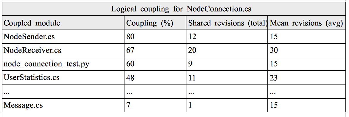
Logical coupling analysis of the module NodeConnection.cs.
Visualizing logical coupling
In its simplest form logical coupling can be visualized by frequency diagrams. But just like the analysis of the organization metrics above it's the overlap between traditional complexity and our more subtle measure of logical coupling that is the main point of interest. Where the two meet, there's likely to be a future refactoring feast. It's a data point we want to stand-out in our visualizations.
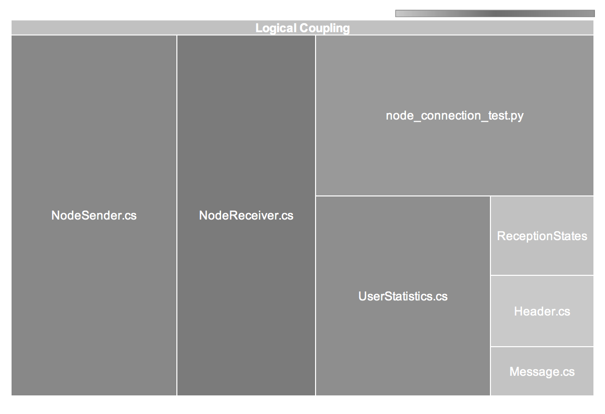
Combined visualization of logical coupling and module complexity using tree maps.
To visualize that multi-dimensional space I use tree maps where each tile represents a module. The size of each tile is proportional to its module's degree of logical coupling. The complexity of the coupled module (e.g. lines of code or Cyclomatic Complexity) is visualized using color mark-up; the darker the color, the more complex the module.
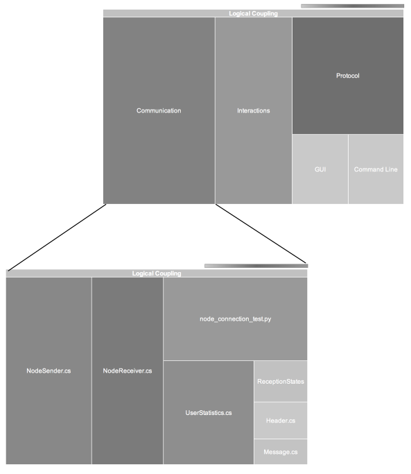
A hierarchical view of the logical coupling partitioned on a per-layer basis.
Tree maps are an excellent choice in cases where the differing sizes or sheer amount of individual components would render a pie chart unreadable. Tree maps are also well-suited to illustrate hierarchical structure. One possible hierarchical visualization is to aggregate the logical coupling over packages and present a multi-layered top-down view of the total coupling in the system as illustrated above.
Whatever we chose, once the logical coupling data is mined, our next step is to find out why specific modules keep changing together.
A couple for a reason
Logical coupling arises for a reason. The most common case is copy-paste code. This one is straightforward to address; extract and encapsulate the common functionality. But logical coupling often have more subtle roots. Perhaps the coupled modules reflect different roles, like a producer and consumer of specific information. In the example above, NodeSender.cs and NodeReceiver.cs seem to reflect those responsibilities. In such case it's not obvious what to do. Perhaps it's not even desirable to change the structure. It's situations like these that require our human expertise to pass an informed judgment within the given context.
The third reason for logical coupling is related to our timeless principles of encapsulation and cohesion. As the data above illustrates, the UserStatistics.cs module changed together with our NodeConnection.cs 48 percent of the time. To me there's no obvious reason it should. To find out why they're coupled we need to take the analysis a step further. Using our VCS data we can dig deeper and start to compare changed lines of code between the coupled files over the common commits. Once we see the pattern of change, it usually suggests there's some smaller module looking to get out. Refactoring towards that goal breaks the logical coupling.
Cases like these teaches us about the design of our system and points-out the direction for improvements. There's much to learn from a logical coupling analysis. Better yet, it's a language neutral technology.
A holistic view by language neutral analysis
VCS data is language neutral. Since our analysis allows us to cross language boundaries, we get a holistic picture of the complete system. In our increasingly polyglot programming world this is a major advantage over traditional software metrics.
Software shops often relay on multiple implementation technologies. One example is using a popular language such as Java or C# for the application development while writing automated tests in a more dynamic language like Python or Ruby. In Table 2 there's an example on this case where node_connection_test.py changes together with the module under test 60 percent of the time. Such a degree of coupling may be expected for a unit test. But in case the Python script serves as an end-to-end test it's probably exposed to way too much implementation detail. Web development is yet another example where a language neutral analysis is beneficial. A VCS-based analysis allows us to spot logical coupling between the document structure (HTML), the dynamic content (JavaScript) and the server software delivering the artifacts (Java, Clojure, Smalltalk, etc).
The road ahead
To understand large-scale software systems we need to look at their evolution. The history of our system provides us with data we cannot derive from a single snapshot of the source code. Instead VCS data blends technical, social and organizational information along a temporal axis that let us map out our interaction patterns in the code. Analyzing these patterns gives us early warnings on potential design issues and development bottlenecks, as well as suggesting new modularities based on actual interactions with the code. Addressing these issues saves costs, simplifies maintenance and let us evolve our systems in the direction of how we actually work with the code.
The road ahead points to a wider application of the techniques. While this article focused on analyzing the design aspect of software, reading code is a harder problem to solve. Integrating analysis of VCS data in the daily workflow of the programmer would allow such a system to provide reading recommendations. For example, “programmers that read the code for the Communication module also checked-out the UserStatistics module” is a likely future recommendation to be seen in your favorite IDE.
Integrating VCS data into our daily workflow would allow future analysis methods to be more fine-grained. There's much improvement to be made if we could consider the time-scale within a single commit. As such, VCS data serves as both feedback and a helpful guide.
Code as a Crime Scene - the book!
Code as a crime scene is an adapted chapter from my upcoming book with the same name. Please check it out for more writings on software design and its psychological aspects.
References
- Canter, D. & Youngs, D. (2008). Principles of Geographical Offender Profiling
- Code City
- D'Ambros, M., Lanza, M. & Lungu, M. (2006). The Evolution Radar
- Fowler, M. (1999). Refactoring
- Glass, R. L. (2002). Facts and Fallacies of Software Engineering
- Glass, R.L. (2006). Software Creativity 2.0
- Halstead, M.H. (1977). Elements of software science
- McCabe, T.J. (1976). A Complexity Measure
- Nagappan, N., Murphy, B. & Basiliet, V. (2008). The influence of organizational structure on software quality